顶点序列的索引方式非常类似于普通的数值型 R 向量,但有一些额外的功能。
多个索引
在括号中使用多个索引时,所有索引都会被独立评估,然后使用 c() 函数连接结果(除了 na_ok 参数,这是一个特殊参数,必须命名)。 例如,V(g)[1, 2, .nei(1)] 等效于 c(V(g)[1], V(g)[2], V(g)[.nei(1)])。
索引类型
顶点序列可以使用正数值向量、负数值向量、逻辑向量、字符向量进行索引。
当使用正数值向量索引时,将选择序列中给定位置的顶点。 这与使用正数值向量索引常规 R 原子向量相同。
当使用负数值向量索引时,将省略序列中给定位置的顶点。 同样,这与索引常规 R 原子向量相同。
当使用逻辑向量索引时,顶点序列的长度和索引的长度必须匹配,并且选择索引为
TRUE的顶点。可以使用字符向量索引命名图,以选择具有给定名称的顶点。
顶点属性
在索引顶点序列时,可以通过使用其名称简单地引用顶点属性。 例如,如果一个图具有 name 顶点属性,则 V(g)[name == "foo"] 等效于 V(g)[V(g)$name == "foo"]。 请参阅下面的更多示例。 请注意,属性名称会屏蔽调用环境中存在的变量的名称; 如果您需要查找变量并且不希望类似命名的顶点属性屏蔽它,请使用 .env 代词在调用环境中执行名称查找。 换句话说,使用 V(g)[.env$name == "foo"] 以确保从调用环境中查找 name,即使存在同名的顶点属性也是如此。 同样,您可以使用 .data 仅匹配属性名称。
特殊函数
有一些特殊的 igraph 函数只能在索引顶点序列的表达式中使用
.nei将顶点序列作为参数,并选择这些顶点的邻居。 可以使用可选的
mode参数在有向图中选择后继 (mode="out") 或前驱 (mode="in")。.inc将边序列作为参数,并选择在此边序列中至少有一条关联边的顶点。
.from类似于
.inc,但只考虑边的尾部。.to类似于
.inc,但只考虑边的头部。.innei,.outnei.innei(v)是.nei(v, mode = "in")的简写形式,而.outnei(v)是.nei(v, mode = "out")的简写形式。
请注意,多个特殊函数可以一起使用,或与常规索引一起使用,然后将它们的结果连接起来。 请参阅下面的更多示例。
参见
其他顶点和边序列: E(), V(), as_ids(), igraph-es-attributes, igraph-es-indexing, igraph-es-indexing2, igraph-vs-attributes, igraph-vs-indexing2, print.igraph.es(), print.igraph.vs()
其他顶点和边序列操作: c.igraph.es(), c.igraph.vs(), difference.igraph.es(), difference.igraph.vs(), igraph-es-indexing, igraph-es-indexing2, igraph-vs-indexing2, intersection.igraph.es(), intersection.igraph.vs(), rev.igraph.es(), rev.igraph.vs(), union.igraph.es(), union.igraph.vs(), unique.igraph.es(), unique.igraph.vs()
示例
# -----------------------------------------------------------------
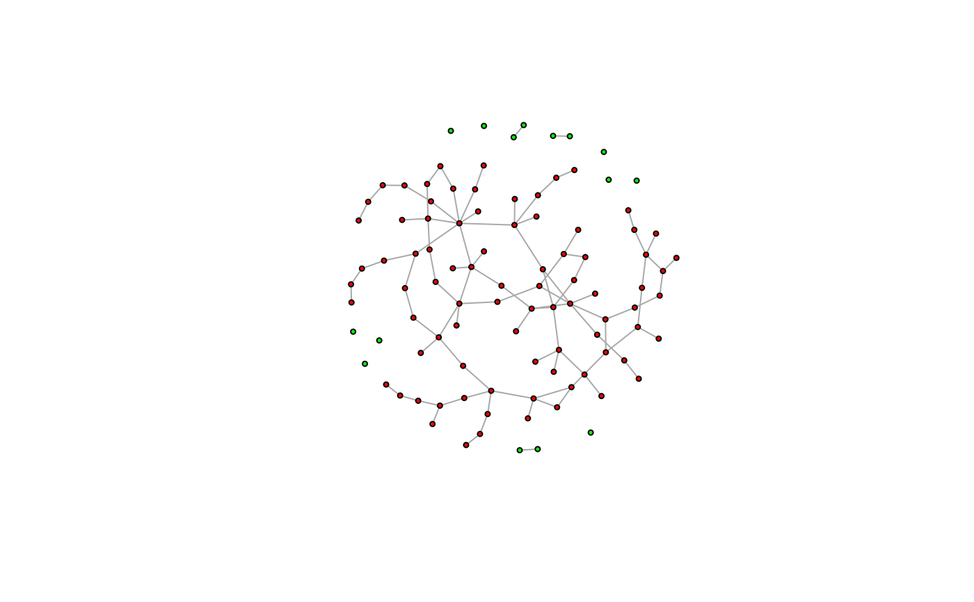
# Setting attributes for subsets of vertices
largest_comp <- function(graph) {
cl <- components(graph)
V(graph)[which.max(cl$csize) == cl$membership]
}
g <- sample_(
gnp(100, 2 / 100),
with_vertex_(size = 3, label = ""),
with_graph_(layout = layout_with_fr)
)
giant_v <- largest_comp(g)
V(g)$color <- "green"
V(g)[giant_v]$color <- "red"
plot(g)
 # -----------------------------------------------------------------
# nei() special function
g <- make_graph(c(1, 2, 2, 3, 2, 4, 4, 2))
V(g)[.nei(c(2, 4))]
#> + 4/4 vertices, from a28d1d5:
#> [1] 1 2 3 4
V(g)[.nei(c(2, 4), "in")]
#> + 3/4 vertices, from a28d1d5:
#> [1] 1 2 4
V(g)[.nei(c(2, 4), "out")]
#> + 3/4 vertices, from a28d1d5:
#> [1] 2 3 4
# -----------------------------------------------------------------
# The same with vertex names
g <- make_graph(~ A -+ B, B -+ C:D, D -+ B)
V(g)[.nei(c("B", "D"))]
#> + 4/4 vertices, named, from deae1e2:
#> [1] A B C D
V(g)[.nei(c("B", "D"), "in")]
#> + 3/4 vertices, named, from deae1e2:
#> [1] A B D
V(g)[.nei(c("B", "D"), "out")]
#> + 3/4 vertices, named, from deae1e2:
#> [1] B C D
# -----------------------------------------------------------------
# Resolving attributes
g <- make_graph(~ A -+ B, B -+ C:D, D -+ B)
V(g)$color <- c("red", "red", "green", "green")
V(g)[color == "red"]
#> + 2/4 vertices, named, from 6e8b170:
#> [1] A B
# Indexing with a variable whose name matches the name of an attribute
# may fail; use .env to force the name lookup in the parent environment
V(g)$x <- 10:13
x <- 2
V(g)[.env$x]
#> + 1/4 vertex, named, from 6e8b170:
#> [1] B
# -----------------------------------------------------------------
# nei() special function
g <- make_graph(c(1, 2, 2, 3, 2, 4, 4, 2))
V(g)[.nei(c(2, 4))]
#> + 4/4 vertices, from a28d1d5:
#> [1] 1 2 3 4
V(g)[.nei(c(2, 4), "in")]
#> + 3/4 vertices, from a28d1d5:
#> [1] 1 2 4
V(g)[.nei(c(2, 4), "out")]
#> + 3/4 vertices, from a28d1d5:
#> [1] 2 3 4
# -----------------------------------------------------------------
# The same with vertex names
g <- make_graph(~ A -+ B, B -+ C:D, D -+ B)
V(g)[.nei(c("B", "D"))]
#> + 4/4 vertices, named, from deae1e2:
#> [1] A B C D
V(g)[.nei(c("B", "D"), "in")]
#> + 3/4 vertices, named, from deae1e2:
#> [1] A B D
V(g)[.nei(c("B", "D"), "out")]
#> + 3/4 vertices, named, from deae1e2:
#> [1] B C D
# -----------------------------------------------------------------
# Resolving attributes
g <- make_graph(~ A -+ B, B -+ C:D, D -+ B)
V(g)$color <- c("red", "red", "green", "green")
V(g)[color == "red"]
#> + 2/4 vertices, named, from 6e8b170:
#> [1] A B
# Indexing with a variable whose name matches the name of an attribute
# may fail; use .env to force the name lookup in the parent environment
V(g)$x <- 10:13
x <- 2
V(g)[.env$x]
#> + 1/4 vertex, named, from 6e8b170:
#> [1] B