根据 Davidson 和 Harel 的模拟退火算法,将图的顶点放置在平面上。
用法
layout_with_dh(
  graph,
  coords = NULL,
  maxiter = 10,
  fineiter = max(10, log2(vcount(graph))),
  cool.fact = 0.75,
  weight.node.dist = 1,
  weight.border = 0,
  weight.edge.lengths = edge_density(graph)/10,
  weight.edge.crossings = 1 - sqrt(edge_density(graph)),
  weight.node.edge.dist = 0.2 * (1 - edge_density(graph))
)

with_dh(...)
参数
- graph
要布局的图。边的方向被忽略。
- 坐标
顶点的可选起始位置。如果此参数不为
NULL,则它应该是一个合适的起始坐标矩阵。- maxiter
第一阶段要执行的迭代次数。
- fineiter
微调阶段的迭代次数。
- cool.fact
冷却因子。
- weight.node.dist
能量函数中节点-节点距离分量的权重。
- weight.border
能量函数中距边界分量的权重。如果允许顶点位于边界上,则可以设置为零。
- weight.edge.lengths
能量函数中边长分量的权重。
- weight.edge.crossings
能量函数中边交叉分量的权重。
- weight.node.edge.dist
能量函数中节点-边距离分量的权重。
- ...
传递给
layout_with_dh()。
详细信息
此函数实现了 Davidson 和 Harel 的算法,请参阅 Ron Davidson, David Harel: Drawing Graphs Nicely Using Simulated Annealing. ACM Transactions on Graphics 15(4), pp. 301-331, 1996。
该算法使用模拟退火和复杂的能量函数,不幸的是,对于不同的图,能量函数很难参数化。原始出版物没有透露任何参数值,下面的参数值是通过实验确定的。
该算法包括两个阶段,一个退火阶段和一个微调阶段。第二阶段没有模拟退火。
我们的实现试图尽可能地遵循原始出版物。唯一的重大区别是坐标被明确地保持在布局矩形的范围内。
参考文献
Ron Davidson, David Harel: Drawing Graphs Nicely Using Simulated Annealing. ACM Transactions on Graphics 15(4), pp. 301-331, 1996.
参见
layout_with_fr(), layout_with_kk() 用于其他布局算法。
其他图布局: add_layout_(), component_wise(), layout_(), layout_as_bipartite(), layout_as_star(), layout_as_tree(), layout_in_circle(), layout_nicely(), layout_on_grid(), layout_on_sphere(), layout_randomly(), layout_with_fr(), layout_with_gem(), layout_with_graphopt(), layout_with_kk(), layout_with_lgl(), layout_with_mds(), layout_with_sugiyama(), merge_coords(), norm_coords(), normalize()
作者
Gabor Csardi csardi.gabor@gmail.com
示例
set.seed(42)
## Figures from the paper
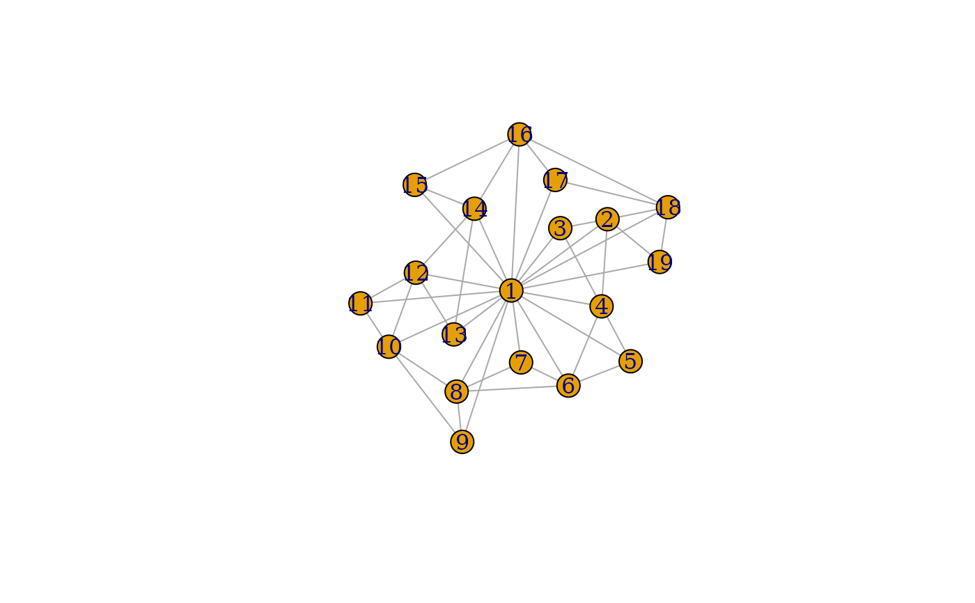
g_1b <- make_star(19, mode = "undirected") + path(c(2:19, 2)) +
path(c(seq(2, 18, by = 2), 2))
plot(g_1b, layout = layout_with_dh)
 g_2 <- make_lattice(c(8, 3)) + edges(1, 8, 9, 16, 17, 24)
plot(g_2, layout = layout_with_dh)
g_2 <- make_lattice(c(8, 3)) + edges(1, 8, 9, 16, 17, 24)
plot(g_2, layout = layout_with_dh)
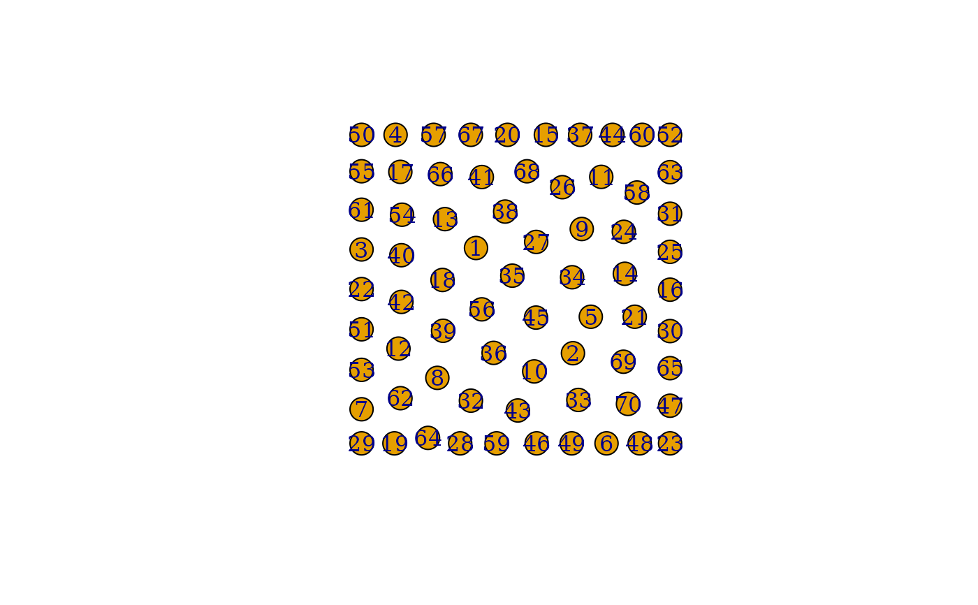
 g_3 <- make_empty_graph(n = 70)
plot(g_3, layout = layout_with_dh)
g_3 <- make_empty_graph(n = 70)
plot(g_3, layout = layout_with_dh)
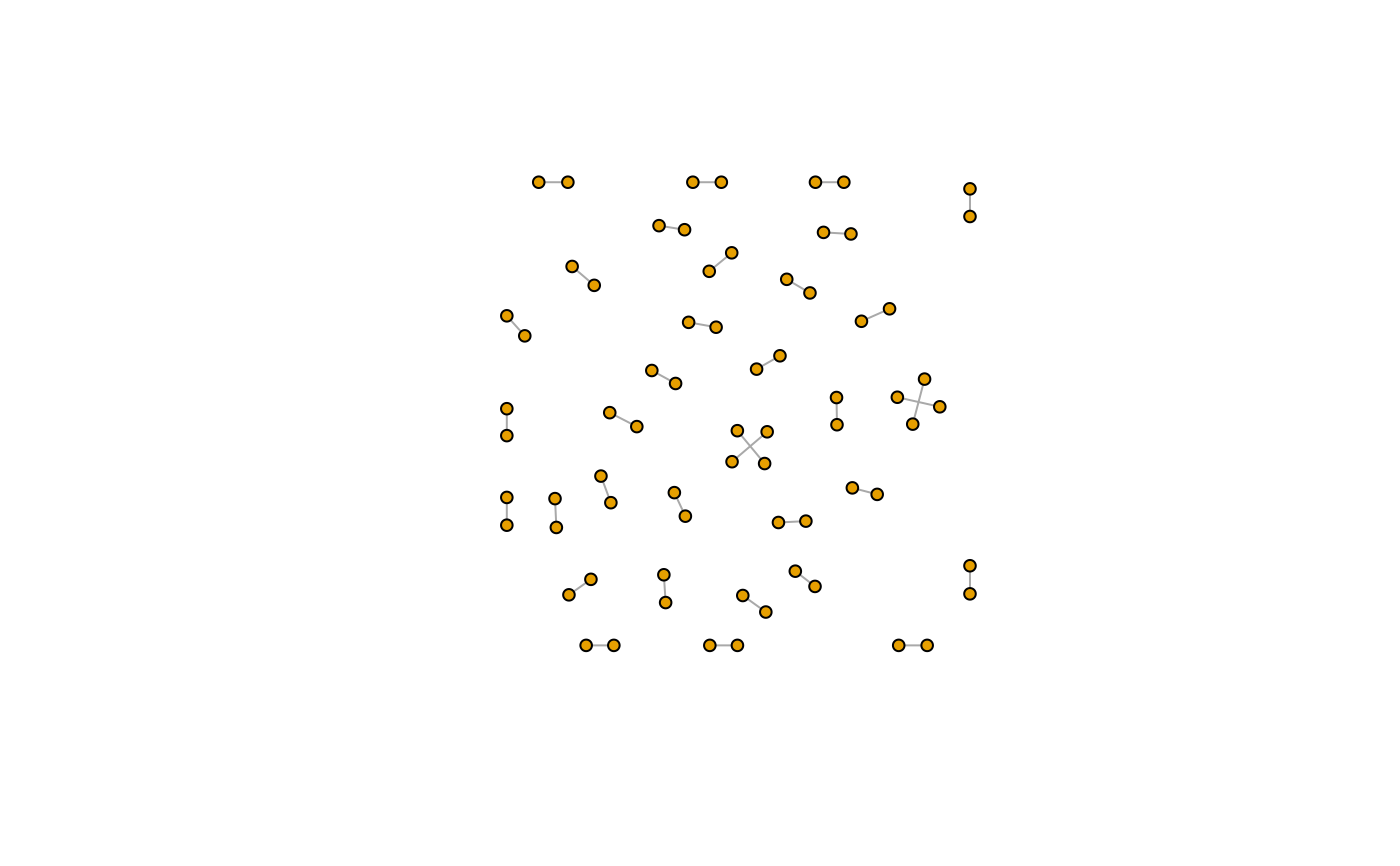
 g_4 <- make_empty_graph(n = 70, directed = FALSE) + edges(1:70)
plot(g_4, layout = layout_with_dh, vertex.size = 5, vertex.label = NA)
g_4 <- make_empty_graph(n = 70, directed = FALSE) + edges(1:70)
plot(g_4, layout = layout_with_dh, vertex.size = 5, vertex.label = NA)
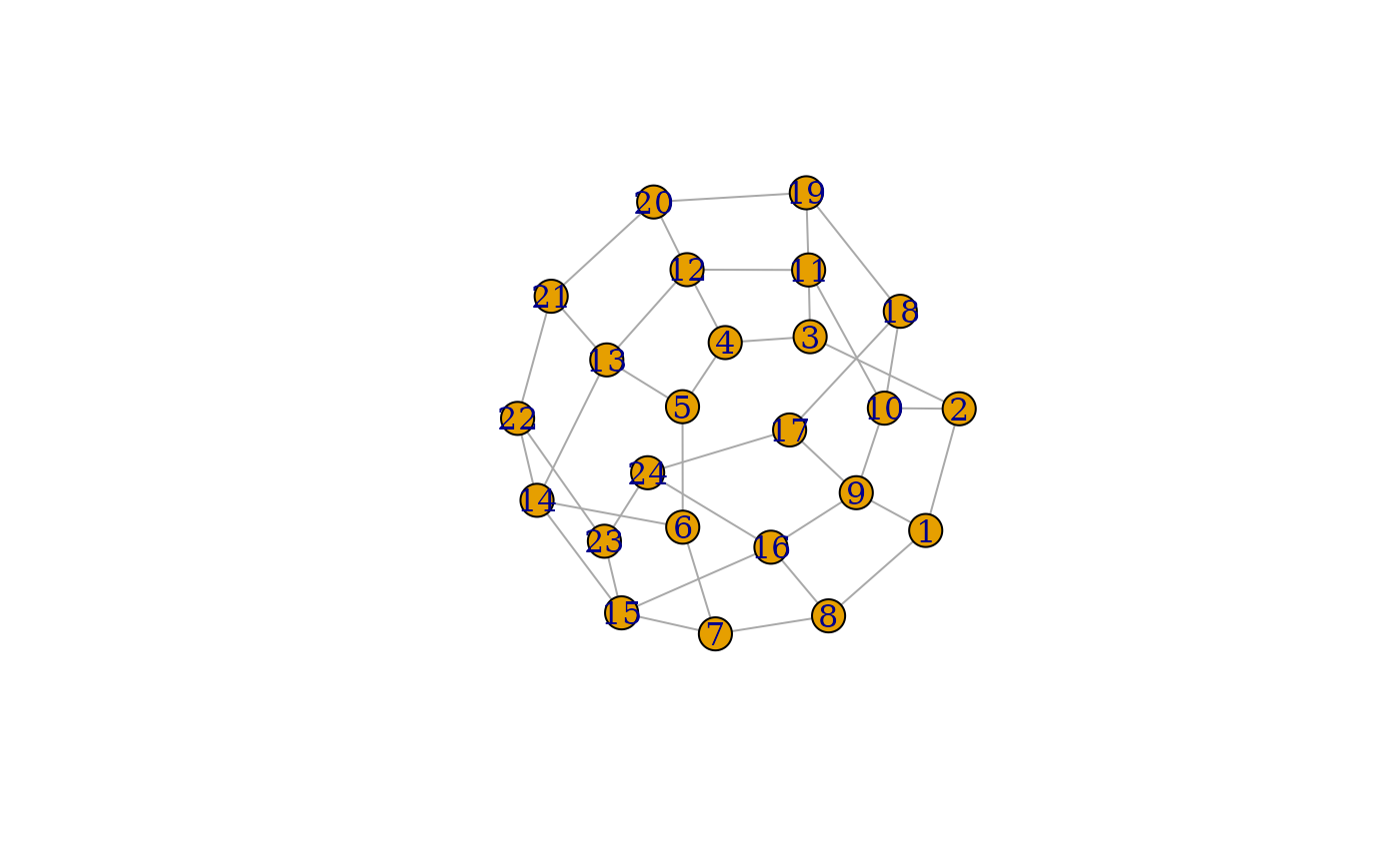
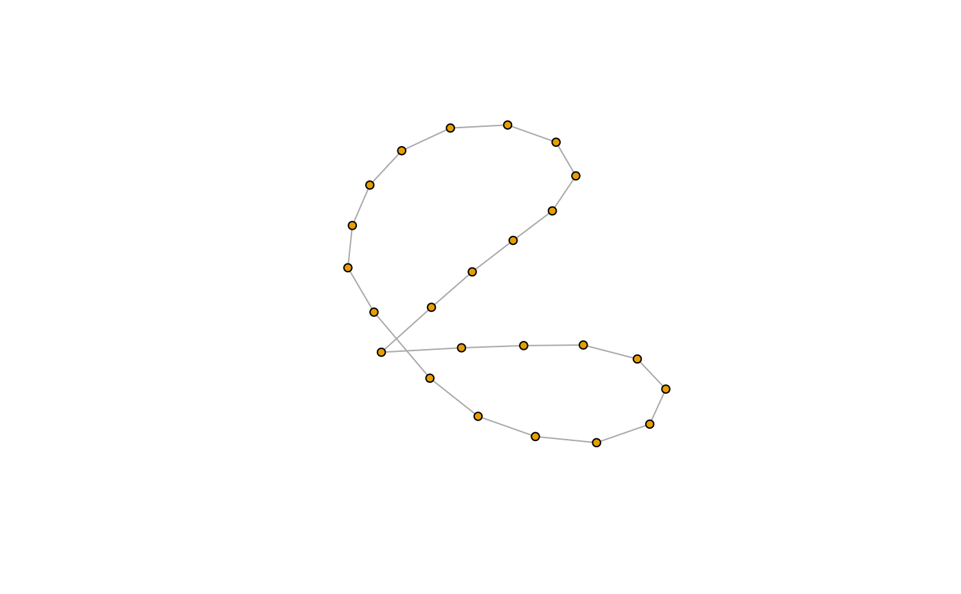
 g_5a <- make_ring(24)
plot(g_5a, layout = layout_with_dh, vertex.size = 5, vertex.label = NA)
g_5a <- make_ring(24)
plot(g_5a, layout = layout_with_dh, vertex.size = 5, vertex.label = NA)
 g_5b <- make_ring(40)
plot(g_5b, layout = layout_with_dh, vertex.size = 5, vertex.label = NA)
g_5b <- make_ring(40)
plot(g_5b, layout = layout_with_dh, vertex.size = 5, vertex.label = NA)
 g_6 <- make_lattice(c(2, 2, 2))
plot(g_6, layout = layout_with_dh)
g_6 <- make_lattice(c(2, 2, 2))
plot(g_6, layout = layout_with_dh)
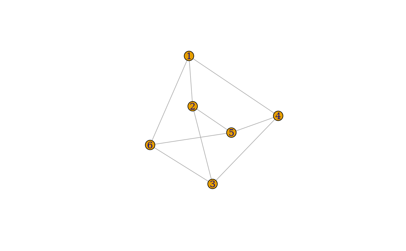
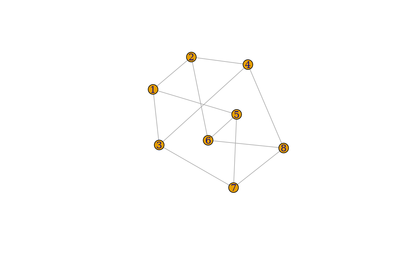 g_7 <- graph_from_literal(1:3:5 - -2:4:6)
plot(g_7, layout = layout_with_dh, vertex.label = V(g_7)$name)
g_7 <- graph_from_literal(1:3:5 - -2:4:6)
plot(g_7, layout = layout_with_dh, vertex.label = V(g_7)$name)
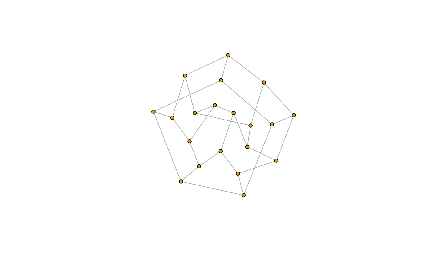
 g_8 <- make_ring(5) + make_ring(10) + make_ring(5) +
edges(
1, 6, 2, 8, 3, 10, 4, 12, 5, 14,
7, 16, 9, 17, 11, 18, 13, 19, 15, 20
)
plot(g_8, layout = layout_with_dh, vertex.size = 5, vertex.label = NA)
g_8 <- make_ring(5) + make_ring(10) + make_ring(5) +
edges(
1, 6, 2, 8, 3, 10, 4, 12, 5, 14,
7, 16, 9, 17, 11, 18, 13, 19, 15, 20
)
plot(g_8, layout = layout_with_dh, vertex.size = 5, vertex.label = NA)
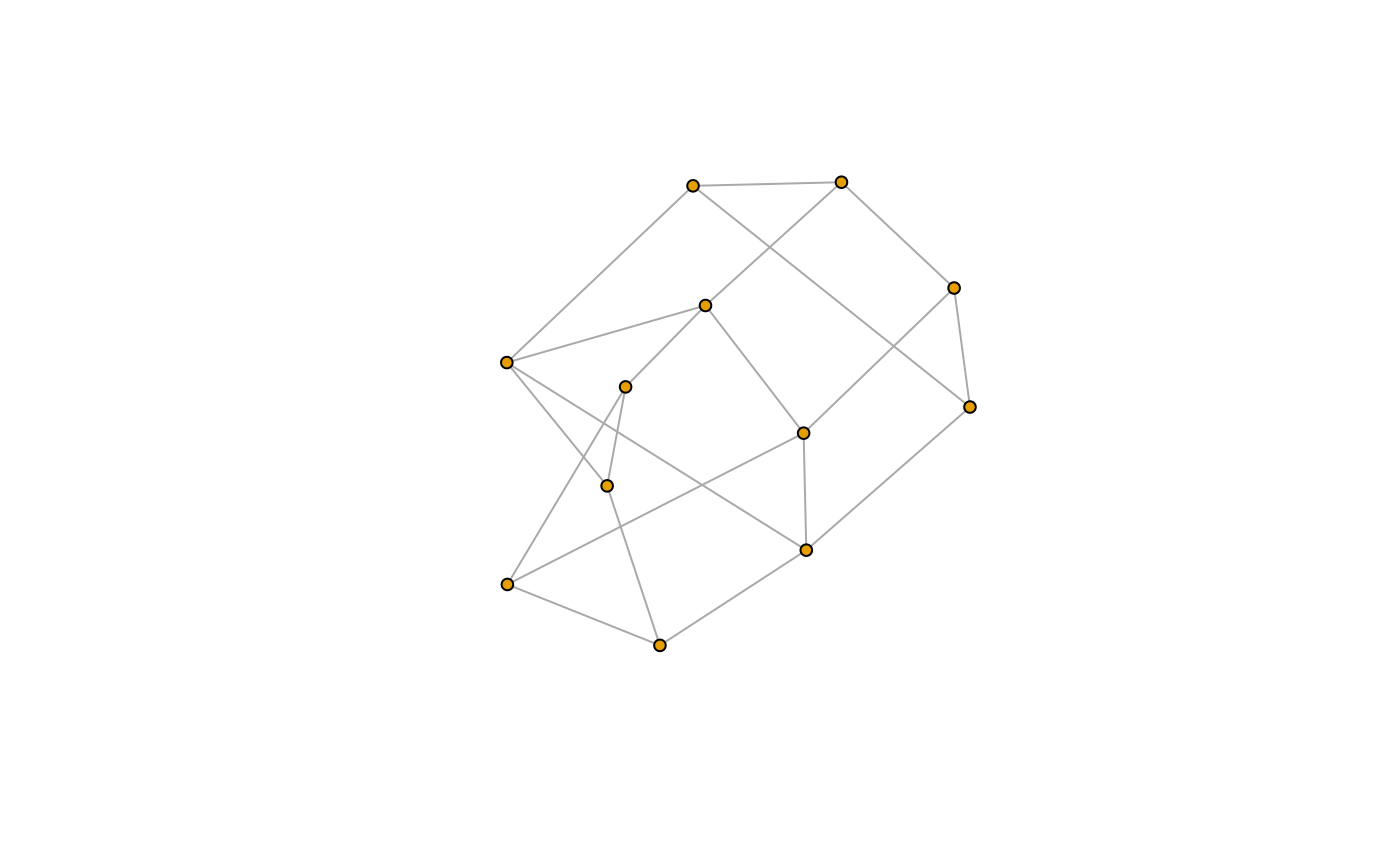
 g_9 <- make_lattice(c(3, 2, 2))
plot(g_9, layout = layout_with_dh, vertex.size = 5, vertex.label = NA)
g_9 <- make_lattice(c(3, 2, 2))
plot(g_9, layout = layout_with_dh, vertex.size = 5, vertex.label = NA)
 g_10 <- make_lattice(c(6, 6))
plot(g_10, layout = layout_with_dh, vertex.size = 5, vertex.label = NA)
g_10 <- make_lattice(c(6, 6))
plot(g_10, layout = layout_with_dh, vertex.size = 5, vertex.label = NA)
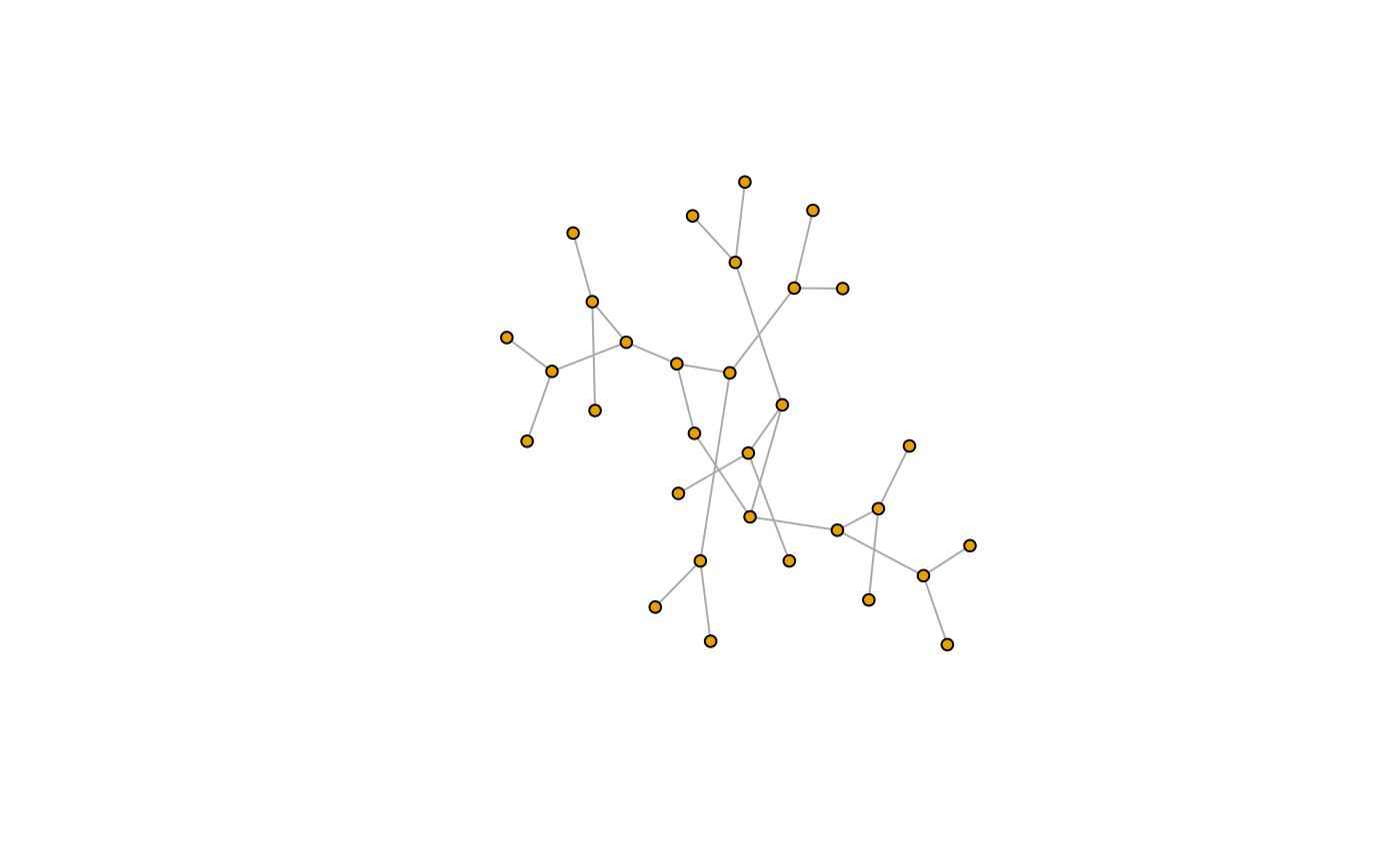
 g_11a <- make_tree(31, 2, mode = "undirected")
plot(g_11a, layout = layout_with_dh, vertex.size = 5, vertex.label = NA)
g_11a <- make_tree(31, 2, mode = "undirected")
plot(g_11a, layout = layout_with_dh, vertex.size = 5, vertex.label = NA)
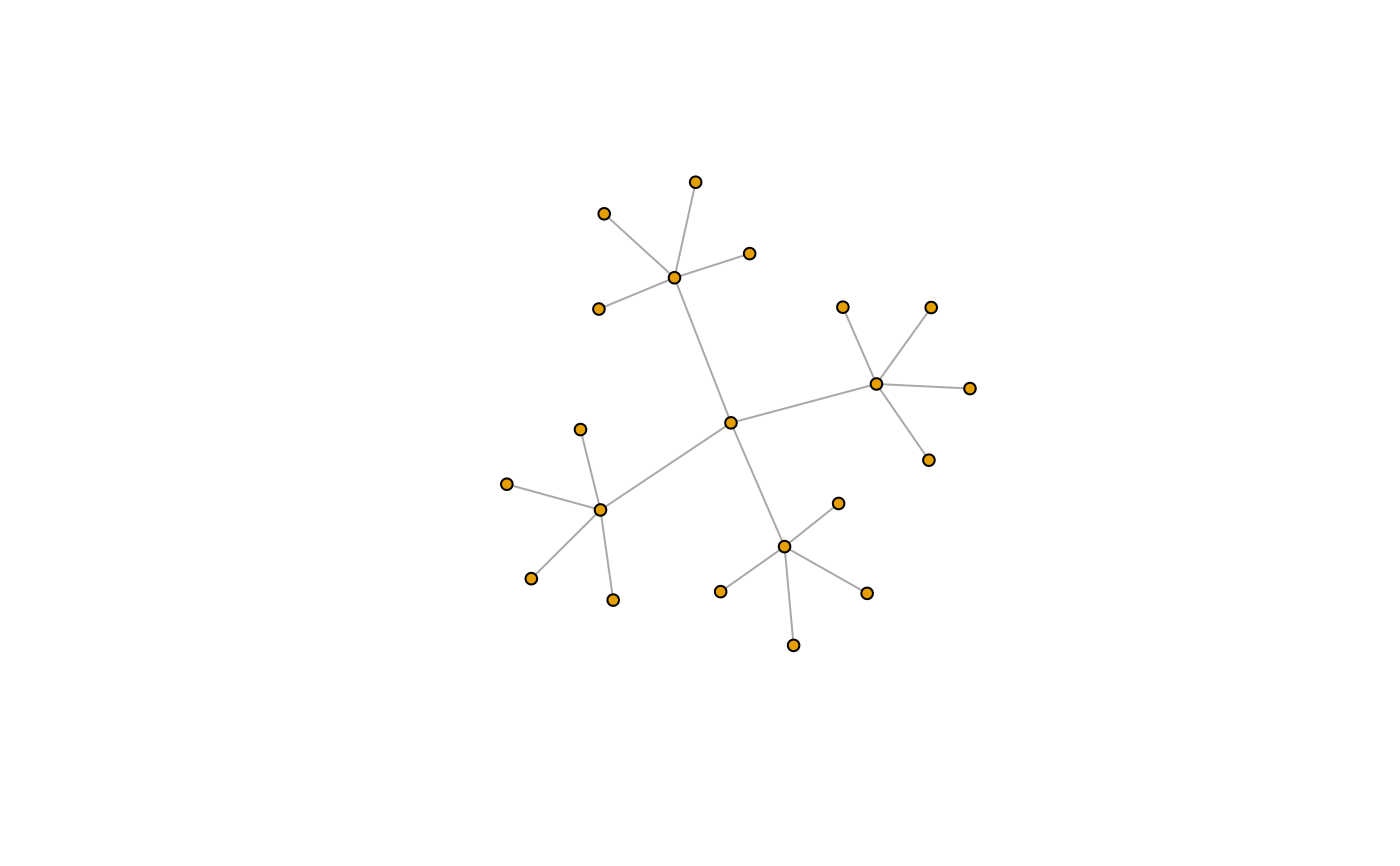
 g_11b <- make_tree(21, 4, mode = "undirected")
plot(g_11b, layout = layout_with_dh, vertex.size = 5, vertex.label = NA)
g_11b <- make_tree(21, 4, mode = "undirected")
plot(g_11b, layout = layout_with_dh, vertex.size = 5, vertex.label = NA)
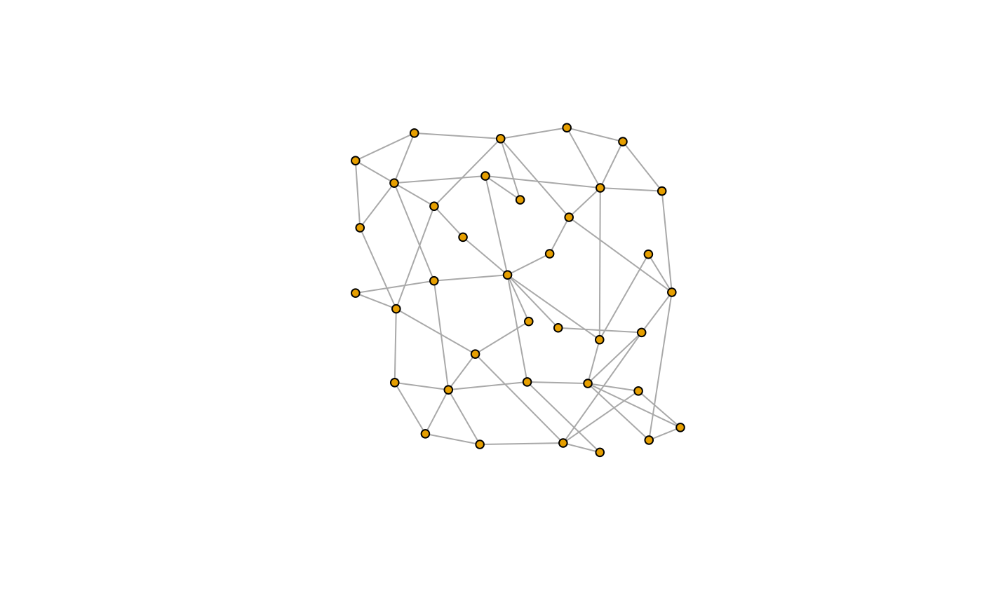
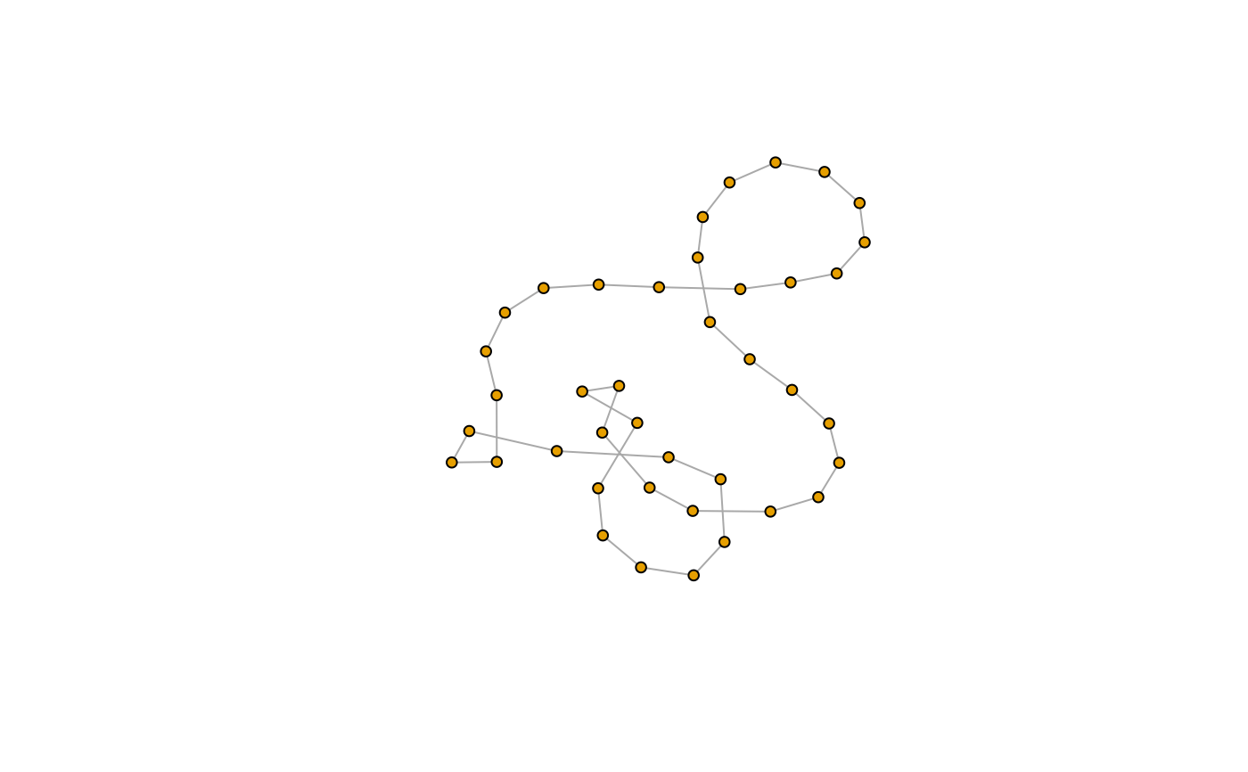
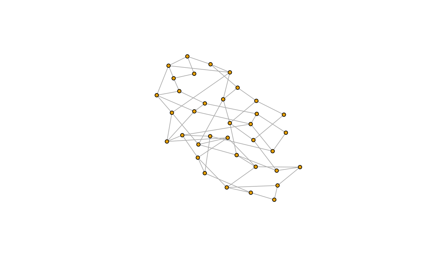
 g_12 <- make_empty_graph(n = 37, directed = FALSE) +
path(1:5, 10, 22, 31, 37:33, 27, 16, 6, 1) + path(6, 7, 11, 9, 10) + path(16:22) +
path(27:31) + path(2, 7, 18, 28, 34) + path(3, 8, 11, 19, 29, 32, 35) +
path(4, 9, 20, 30, 36) + path(1, 7, 12, 14, 19, 24, 26, 30, 37) +
path(5, 9, 13, 15, 19, 23, 25, 28, 33) + path(3, 12, 16, 25, 35, 26, 22, 13, 3)
plot(g_12, layout = layout_with_dh, vertex.size = 5, vertex.label = NA)
g_12 <- make_empty_graph(n = 37, directed = FALSE) +
path(1:5, 10, 22, 31, 37:33, 27, 16, 6, 1) + path(6, 7, 11, 9, 10) + path(16:22) +
path(27:31) + path(2, 7, 18, 28, 34) + path(3, 8, 11, 19, 29, 32, 35) +
path(4, 9, 20, 30, 36) + path(1, 7, 12, 14, 19, 24, 26, 30, 37) +
path(5, 9, 13, 15, 19, 23, 25, 28, 33) + path(3, 12, 16, 25, 35, 26, 22, 13, 3)
plot(g_12, layout = layout_with_dh, vertex.size = 5, vertex.label = NA)