用于分层有向无环图的 Sugiyama 布局算法。该算法最小化边交叉。
用法
layout_with_sugiyama(
  graph,
  layers = NULL,
  hgap = 1,
  vgap = 1,
  maxiter = 100,
  weights = NULL,
  attributes = c("default", "all", "none")
)

with_sugiyama(...)
参数
- graph
输入图。
- layers
一个数值向量或
NULL。如果不是NULL,则应指定顶点的层索引。层从一开始编号。如果是NULL,则 igraph 会自动计算层。- hgap
实数标量,同一层中顶点之间的最小水平间隙。
- vgap
实数标量,层之间的距离。
- maxiter
整数标量,交叉最小化阶段的最大迭代次数。100 是一个合理的默认值;如果您觉得边交叉过多,请增加此值。
- weights
可选的边权重向量。如果是
NULL,则使用 'weight' 边属性(如果存在)。在此处提供NA,igraph 将忽略边权重。这些仅在图包含循环时使用;igraph 在打破循环时会倾向于反转权重较小的边。- attributes
要在扩展图中保留哪些图/顶点/边属性。“default”保留“size”、“size2”、“shape”、“label”和“color”顶点属性以及“arrow.mode”和“arrow.size”边属性。“all”保留所有图、顶点和边属性,“none”不保留任何属性。
- ...
传递给
layout_with_sugiyama()。
值
具有以下组件的列表
- layout
原始图顶点的布局,一个两列矩阵。
- layout.dummy
虚拟顶点的布局,一个两列矩阵。
- extd_graph
原始图,用虚拟顶点扩展。“dummy”顶点属性在此图上设置,它是一个逻辑属性,告诉您该顶点是否为虚拟顶点。“layout”图属性也已设置,它是所有(原始和虚拟)顶点的布局矩阵。
详细信息
此布局算法专为有向无环图设计,其中每个顶点都分配到一个层。层从零开始索引,同一层的顶点将放置在同一水平线上。每个层中顶点的 X 坐标由 Sugiyama 等人提出的启发式方法决定,以最小化边交叉。
您也可以尝试使用此算法来布局无向图、包含循环的图或没有先验分层分配的图。 igraph 会尝试消除循环并将顶点分配到层,但不保证在这种情况下布局的质量。
Sugiyama 布局可能会在边上引入“弯曲”,以获得视觉上更令人愉悦的布局。这是通过向跨越多个层的边添加虚拟节点来实现的。生成的布局不仅为原始图的节点分配坐标,还为虚拟节点分配坐标。布局算法还将返回带有虚拟节点的扩展图。
有关更多详细信息,请参阅下面的参考资料。
参考文献
K. Sugiyama, S. Tagawa and M. Toda, "Methods for Visual Understanding of Hierarchical Systems". IEEE Transactions on Systems, Man and Cybernetics 11(2):109-125, 1981.
参见
其他图布局:add_layout_(), component_wise(), layout_(), layout_as_bipartite(), layout_as_star(), layout_as_tree(), layout_in_circle(), layout_nicely(), layout_on_grid(), layout_on_sphere(), layout_randomly(), layout_with_dh(), layout_with_fr(), layout_with_gem(), layout_with_graphopt(), layout_with_kk(), layout_with_lgl(), layout_with_mds(), merge_coords(), norm_coords(), normalize()
作者
Tamas Nepusz ntamas@gmail.com
示例
## Data taken from http://tehnick-8.narod.ru/dc_clients/
DC <- graph_from_literal(
"DC++" -+ "LinuxDC++":"BCDC++":"EiskaltDC++":"StrongDC++":"DiCe!++",
"LinuxDC++" -+ "FreeDC++", "BCDC++" -+ "StrongDC++",
"FreeDC++" -+ "BMDC++":"EiskaltDC++",
"StrongDC++" -+ "AirDC++":"zK++":"ApexDC++":"TkDC++",
"StrongDC++" -+ "StrongDC++ SQLite":"RSX++",
"ApexDC++" -+ "FlylinkDC++ ver <= 4xx",
"ApexDC++" -+ "ApexDC++ Speed-Mod":"DiCe!++",
"StrongDC++ SQLite" -+ "FlylinkDC++ ver >= 5xx",
"ApexDC++ Speed-Mod" -+ "FlylinkDC++ ver <= 4xx",
"ApexDC++ Speed-Mod" -+ "GreylinkDC++",
"FlylinkDC++ ver <= 4xx" -+ "FlylinkDC++ ver >= 5xx",
"FlylinkDC++ ver <= 4xx" -+ AvaLink,
"GreylinkDC++" -+ AvaLink:"RayLinkDC++":"SparkDC++":PeLink
)
## Use edge types
E(DC)$lty <- 1
E(DC)["BCDC++" %->% "StrongDC++"]$lty <- 2
E(DC)["FreeDC++" %->% "EiskaltDC++"]$lty <- 2
E(DC)["ApexDC++" %->% "FlylinkDC++ ver <= 4xx"]$lty <- 2
E(DC)["ApexDC++" %->% "DiCe!++"]$lty <- 2
E(DC)["StrongDC++ SQLite" %->% "FlylinkDC++ ver >= 5xx"]$lty <- 2
E(DC)["GreylinkDC++" %->% "AvaLink"]$lty <- 2
## Layers, as on the plot
layers <- list(
c("DC++"),
c("LinuxDC++", "BCDC++"),
c("FreeDC++", "StrongDC++"),
c(
"BMDC++", "EiskaltDC++", "AirDC++", "zK++", "ApexDC++",
"TkDC++", "RSX++"
),
c("StrongDC++ SQLite", "ApexDC++ Speed-Mod", "DiCe!++"),
c("FlylinkDC++ ver <= 4xx", "GreylinkDC++"),
c(
"FlylinkDC++ ver >= 5xx", "AvaLink", "RayLinkDC++",
"SparkDC++", "PeLink"
)
)
## Check that we have all nodes
all(sort(unlist(layers)) == sort(V(DC)$name))
#> [1] TRUE
## Add some graphical parameters
V(DC)$color <- "white"
V(DC)$shape <- "rectangle"
V(DC)$size <- 20
V(DC)$size2 <- 10
V(DC)$label <- lapply(V(DC)$name, function(x) {
paste(strwrap(x, 12), collapse = "\n")
})
E(DC)$arrow.size <- 0.5
## Create a similar layout using the predefined layers
lay1 <- layout_with_sugiyama(DC, layers = apply(sapply(
layers,
function(x) V(DC)$name %in% x
), 1, which))
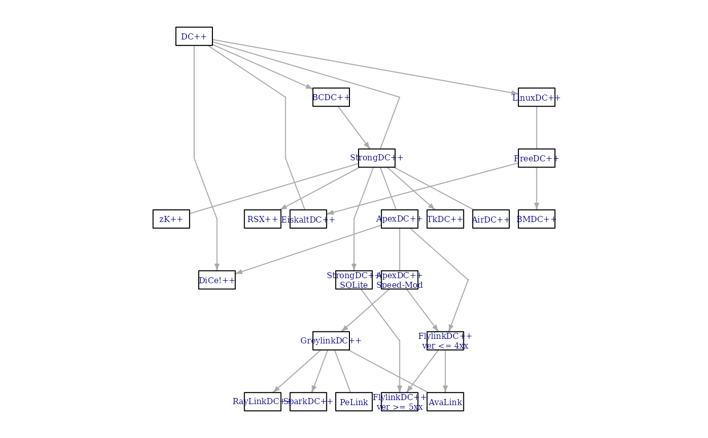
## Simple plot, not very nice
par(mar = rep(.1, 4))
plot(DC, layout = lay1$layout, vertex.label.cex = 0.5)
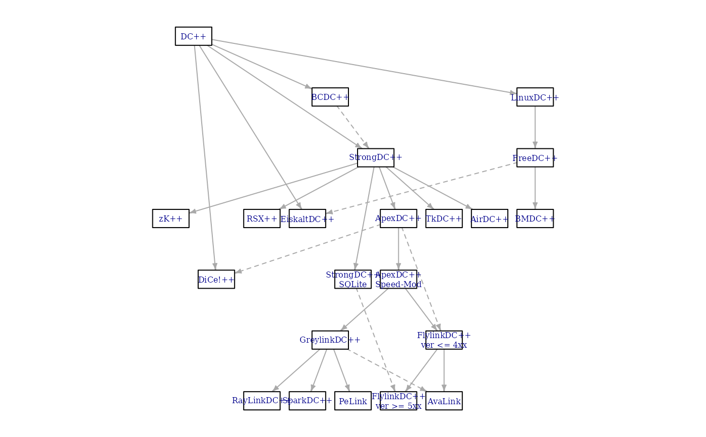 ## Sugiyama plot
plot(lay1$extd_graph, vertex.label.cex = 0.5)
## Sugiyama plot
plot(lay1$extd_graph, vertex.label.cex = 0.5)
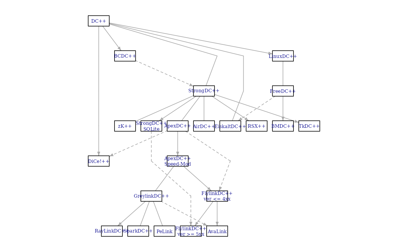
 ## The same with automatic layer calculation
## Keep vertex/edge attributes in the extended graph
lay2 <- layout_with_sugiyama(DC, attributes = "all")
plot(lay2$extd_graph, vertex.label.cex = 0.5)
## The same with automatic layer calculation
## Keep vertex/edge attributes in the extended graph
lay2 <- layout_with_sugiyama(DC, attributes = "all")
plot(lay2$extd_graph, vertex.label.cex = 0.5)
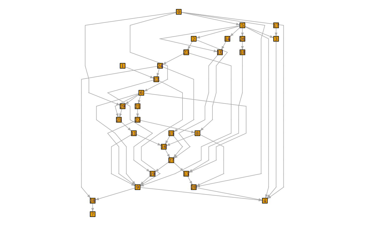
 ## Another example, from the following paper:
## Markus Eiglsperger, Martin Siebenhaller, Michael Kaufmann:
## An Efficient Implementation of Sugiyama's Algorithm for
## Layered Graph Drawing, Journal of Graph Algorithms and
## Applications 9, 305--325 (2005).
ex <- graph_from_literal(
0 -+ 29:6:5:20:4,
1 -+ 12,
2 -+ 23:8,
3 -+ 4,
4,
5 -+ 2:10:14:26:4:3,
6 -+ 9:29:25:21:13,
7,
8 -+ 20:16,
9 -+ 28:4,
10 -+ 27,
11 -+ 9:16,
12 -+ 9:19,
13 -+ 20,
14 -+ 10,
15 -+ 16:27,
16 -+ 27,
17 -+ 3,
18 -+ 13,
19 -+ 9,
20 -+ 4,
21 -+ 22,
22 -+ 8:9,
23 -+ 9:24,
24 -+ 12:15:28,
25 -+ 11,
26 -+ 18,
27 -+ 13:19,
28 -+ 7,
29 -+ 25
)
layers <- list(
0, c(5, 17), c(2, 14, 26, 3), c(23, 10, 18), c(1, 24),
12, 6, c(29, 21), c(25, 22), c(11, 8, 15), 16, 27, c(13, 19),
c(9, 20), c(4, 28), 7
)
layex <- layout_with_sugiyama(ex, layers = apply(
sapply(
layers,
function(x) V(ex)$name %in% as.character(x)
),
1, which
))
origvert <- c(rep(TRUE, vcount(ex)), rep(FALSE, nrow(layex$layout.dummy)))
realedge <- as_edgelist(layex$extd_graph)[, 2] <= vcount(ex)
plot(layex$extd_graph,
vertex.label.cex = 0.5,
edge.arrow.size = .5,
vertex.size = ifelse(origvert, 5, 0),
vertex.shape = ifelse(origvert, "square", "none"),
vertex.label = ifelse(origvert, V(ex)$name, ""),
edge.arrow.mode = ifelse(realedge, 2, 0)
)
## Another example, from the following paper:
## Markus Eiglsperger, Martin Siebenhaller, Michael Kaufmann:
## An Efficient Implementation of Sugiyama's Algorithm for
## Layered Graph Drawing, Journal of Graph Algorithms and
## Applications 9, 305--325 (2005).
ex <- graph_from_literal(
0 -+ 29:6:5:20:4,
1 -+ 12,
2 -+ 23:8,
3 -+ 4,
4,
5 -+ 2:10:14:26:4:3,
6 -+ 9:29:25:21:13,
7,
8 -+ 20:16,
9 -+ 28:4,
10 -+ 27,
11 -+ 9:16,
12 -+ 9:19,
13 -+ 20,
14 -+ 10,
15 -+ 16:27,
16 -+ 27,
17 -+ 3,
18 -+ 13,
19 -+ 9,
20 -+ 4,
21 -+ 22,
22 -+ 8:9,
23 -+ 9:24,
24 -+ 12:15:28,
25 -+ 11,
26 -+ 18,
27 -+ 13:19,
28 -+ 7,
29 -+ 25
)
layers <- list(
0, c(5, 17), c(2, 14, 26, 3), c(23, 10, 18), c(1, 24),
12, 6, c(29, 21), c(25, 22), c(11, 8, 15), 16, 27, c(13, 19),
c(9, 20), c(4, 28), 7
)
layex <- layout_with_sugiyama(ex, layers = apply(
sapply(
layers,
function(x) V(ex)$name %in% as.character(x)
),
1, which
))
origvert <- c(rep(TRUE, vcount(ex)), rep(FALSE, nrow(layex$layout.dummy)))
realedge <- as_edgelist(layex$extd_graph)[, 2] <= vcount(ex)
plot(layex$extd_graph,
vertex.label.cex = 0.5,
edge.arrow.size = .5,
vertex.size = ifelse(origvert, 5, 0),
vertex.shape = ifelse(origvert, "square", "none"),
vertex.label = ifelse(origvert, V(ex)$name, ""),
edge.arrow.mode = ifelse(realedge, 2, 0)
)